Microwave Radar System

Introduction

Over time I have worked with dozens if not hundreds of different electronic sensors for many different environmental factors. Of all the different types of sensors I have used, those that sense distance have always been my favorite. However, in the past I have been limited to store-bought sensors such as the generic HC-SR04 ultrasonic ranging sensor if I needed something cheap and easy and the SHARP GP2Y0A21YK infrared ranging sensor if I had some extra money to spend and needed a more accurate measurement. I wanted to play with the holy grail of distance sensors, a radio detection and ranging (radar) sensor.

Radar has been experimented with since the early 1900s and has existed in its somewhat modern form since the mid 1930s when Robert Watson-Watt used a surplus short-wave BBC radio transmitter to locate a HP.50 Heyford RAF heavy bomber in February 1935. I wanted to make something that had similar functionality to this but more accurate and smaller scale.

Rationale

In recent years there have been a variety of different radar sensors like this one from OmniPreSense but I am not particularly fond of devices like this. Firstly, I think they are somewhat wasteful. For example, suppose I wanted to make one of those LED smart speed limit signs using this device. I would have to attach some sort of microcontroller to this radar, write code to allow it to communicate with it using UART, RS-232 or USB, interpret this data then display it to the LED display. This is all despite the fact that the onboard processor on the radar, an Infineon XMC4500 ARM Cortex M4 microcontroller, could easily control the LED sign without needing any sort of external computers, saving cost, failure points and complexity. Beyond this, I have never made any sort of serious analog device, especially one dealing with high frequencies, and I would love to have the experience of building something like this and interfacing it with modern digital electronics.

By building my own system I also had control over what parts and performance I would get. I could tailor make the device with parts that allow it to operate with, for example, 30 cm of accuracy for 30 meters. The device I actually ended up creating, had much less thought but into it due, in no small part to my lack of experience when I created it, but I feel confident that future versions could be made to much more specific constraints if needed.

My Project

Radar systems function in principle by transmitting radio waves and seeing how long they take to return to the point where they were transmitted. Because radio waves travel at the speed of light, the time they take to return to where they were transmitted is relatively constant. My system operates between ~2.3 GHz and ~2.5GHz. It operates on this band because components are cheap due to 2.4GHz components being available for communications and these frequencies propagating well enough for most things. Unfortunately, there is a good amount of interference on these bands in our modern worlds so some readings can be ruined by someone’s cell phone, microwave or smart toaster transmitting something.

The type of radar I have designed is a frequency modulated continuous wave synthetic aperture radar system. Below I will break down what this means.

Continuous Wave (CW):

Continuous wave means that the radar system is perpetually transmitting a signal. Older radar systems released what is called a “chirp” signal of radio waves then waited for the “chirp” to return before transmitting another chirp. Modern radars rely on continuous wave systems because they are easier to construct and perpetually receive data instead of only gathering it sometimes. Data from an object is gathered by observing how much the received signals’ frequency differs from that of the transmitted signal. By transmitting on a single frequency a frequency shift is created only by moving objects as a result of the Doppler effect. This creates a speed-sensing or “Doppler radar.” If distance measurements are wanted (like what I wanted) then you need to frequency modulate the transmit signal.

Frequency Modulated (FM):

Frequency modulation means that the transmitted signal from the radar changes over time in a predictable way. Assuming you are operating a continuous wave radar, you can vary the frequency based on a certain stable wave form. When this is done instead of the frequency of the received signal changing only based upon the velocity of an object it will now differ based on the time it is transmitted. As explained above, if you know the time a signal was transmitted and the time it took to get back then you can figure out the distance to that object. This is done simply by checking the difference in frequency between the transmitted and received signals. The distance to an object can be determined by processing these signal differences in software. In my implementation of radar the frequency modulation can be toggled on and off by a switch in case a Doppler radar is desired.

Synthetic Aperture:

Synthetic aperture simply means that the aperture (field of view) of the radar can be artificially changed. This basically means that the radar, if placed on a stepper motor rotating at a given speed or on the back of a car moving at a constant rate, can take images of an area based on how far objects are away from it. Currently, the data needs to be processed later to form a synthetic aperture image, however, in the future I would like to use something like the IMU that I programmed for my Raspberry Pi Zero Quadcopter to track and form images in real time similar to what Michael Scarito spoke briefly about in his DEFCON talk.

Inspirations

Anyone who is familiar with the MIT Open Courseware FM CW radar will see that my design is heavily inspired by their design, however I have not used screw-together components from Mini-Circuits and instead opted for a surface mount design to compact the design, reduce RF interference and reduce cost. I also modernized many parts of their design including using newer, more available parts, making it operate on a single +5 volts supply, removing the need for a PC sound card for data acquisition, and changing the antennas from simple tapped waveguide antennas to CNC cut yagi antennas inside smaller waveguides that should have better performance at a smaller size.

Electrical Design

Before I began designing the circuit I created a block diagram that I used to model the circuit. It starts at the ramp waveform generator which I figured would be made up of an op-amp (I actually made a short video documenting this circuit in case you need it for something.) This ramp is fed into a high frequency oscillator that serves as the “local oscillator” of the system (analogous to the carrier frequency in telecommunications systems) which generates the frequency that is eventually transmitted. The frequency is then split by a power divider to create two signals, one that is transmitted and another that is used as a reference for mixing later. The first of these signals is fed into an attenuator (not show in the diagram but needed to ensure that the oscillator power is not inadvertently too high) then a RF amplifier before being fed into the transmit antenna. The signal leaves the transmit antenna, hits an object, and is bounced back to the receive antenna, this signal is again amplified by a RF amplifier and compared to the signal being currently transmitted. The difference between these signals is then fed into the video amplifier that, despite it’s name, does not amplify video but instead the signal coming from the mixer. The amplified mixer signal, as well as the original ramp waveform is provided to the computer so that it can do its signal processing.

I continued by creating a circuit that is based on the following selection of parts:

• Raltron RQRA-2328-2536-CR VCO - high frequency RF oscillator
• KYOCERA AVX AT 0603 Attenuator (3db) - RF attenuator
• NXP BGU8052 - RF amplifier
• Analog Devices HMC213BMS8E - RF mixer
• LMC6484 - video amplifier and ramp waveform generator

If you are familiar with analog electronics then the schematic that I made should be pretty easy to figure out. If you are not familiar with analog electronics this is not the place to learn, catch up on it by watching something like David’s “fundamentals” series on EEVBlog. One signal is simply piped from component to component as I explained before. Any circuitry surrounding the RF components (listed above) are manufacturer recommended setups for the integrated circuits. As I mentioned above I designed the triangle oscillator used for the ramp waveform generator. The video amp is a modified version of the one developed by MIT for their Open Courseware radar.

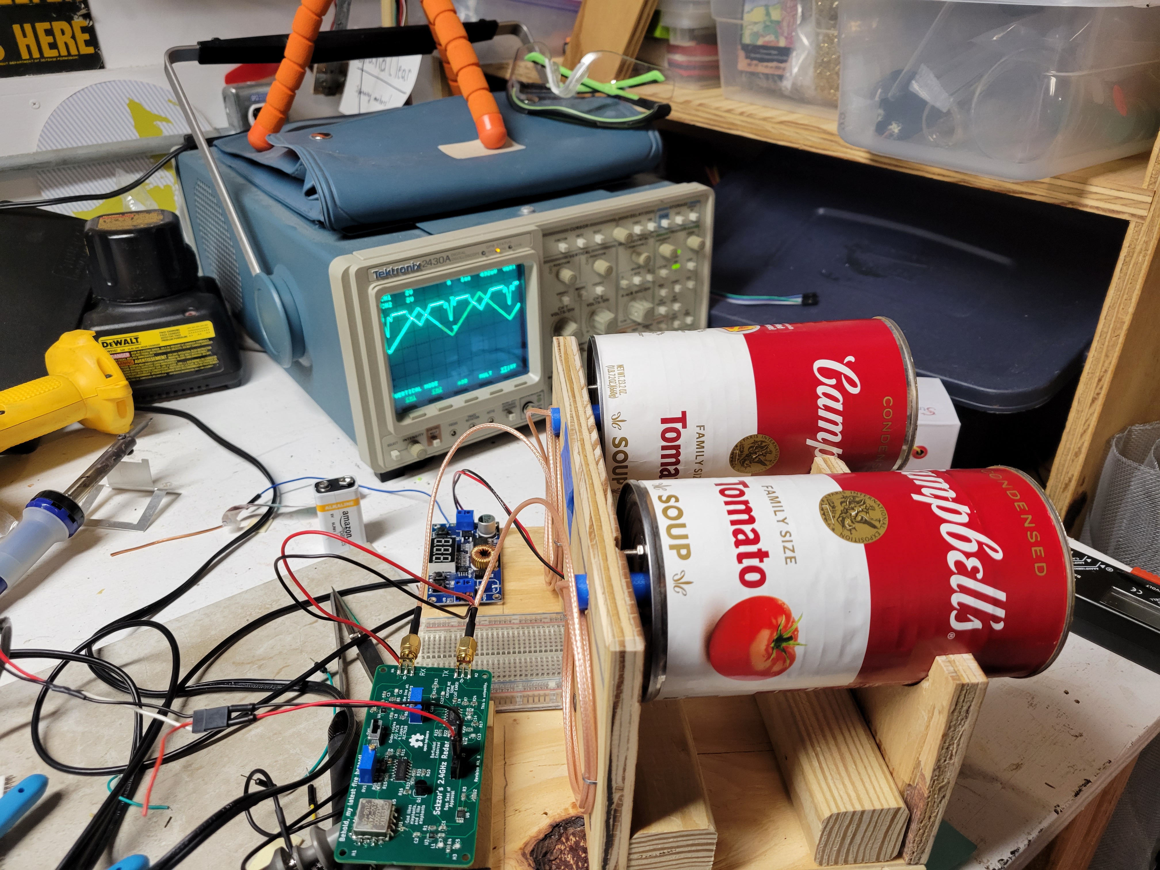
When working on this radar one thing I failed to consider initially is how sensitive the device is to tiny fluctuations in the power lines. The RF mixer for example is not internally amplified, this means that the output voltage of the component seems to hover between 20 millivolts and 100 millivolts. This means that any tiny voltage fluctuation in a switch mode power supply can and do cause significant interference on the output signal. Currently I am using batteries to get around this issue but it would be nice to develop a very stable power supply for use with it. PCBs

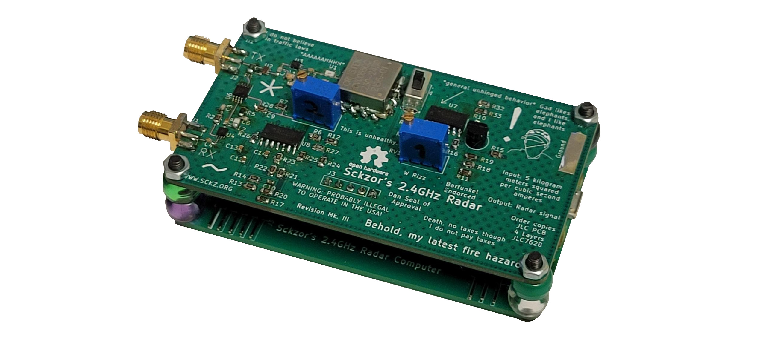
When working on the design of my radar I chose to split the system into 2 printed circuit boards (PCBs). The first contains the analog radar system that actually transmits, receives and compares the radio signals. The second board contains a Raspberry Pi Pico and various supporting circuitry that is used to monitor the modulation and received difference signals coming from the analog radar, perform mathematical filter on them, and either forward them on to a more complicated computer or control some other device based on the signals.

I started by designing the analog radar PCB for the project. This was my first time designing a somewhat complex PCB as well as my first time designing an RF PCB. At the time of writing I have gone through three different designs of the PCB for this project.

Although I have designed different PCBs in the past this one was different because it involved working with RF components. Without going into too much detail, there are certain requirements that must be taken into account when working with frequencies over about 100 MHz. If you are not careful to match the impedance of all of the RF components on the board (including the traces), the components can reflect or distort different signals that pass through them. Additionally, runs between components must be kept to a minimum because long lengths of copper tend to act as antennas when placed near broadcasting RF systems like those that have to exist for radar to exits.

When I first designed the PCB I drew some components footprints without checking if the pad images were front transparent views or rear views of the chip. For this reason some of the pads ended up as mirror images of what they should be. This also means that the first and second were nearly identical. I didn’t feel the need to picture both of the PCBs so above is a photo of the circuit design for the second one. Once the footprint errors were corrected the PCB functioned but it suffered from large interference issues. I do not have access to expensive RF profiling equipment but my best guess as to what the issue was (with the basic bodge wire testing I did) is that the long trace that runs from the receive amplifier to the RF mixer was too long and it was acting as an antenna causing fluctuations in the signal. I attempted to solve these issues with the third revision of the PCB.

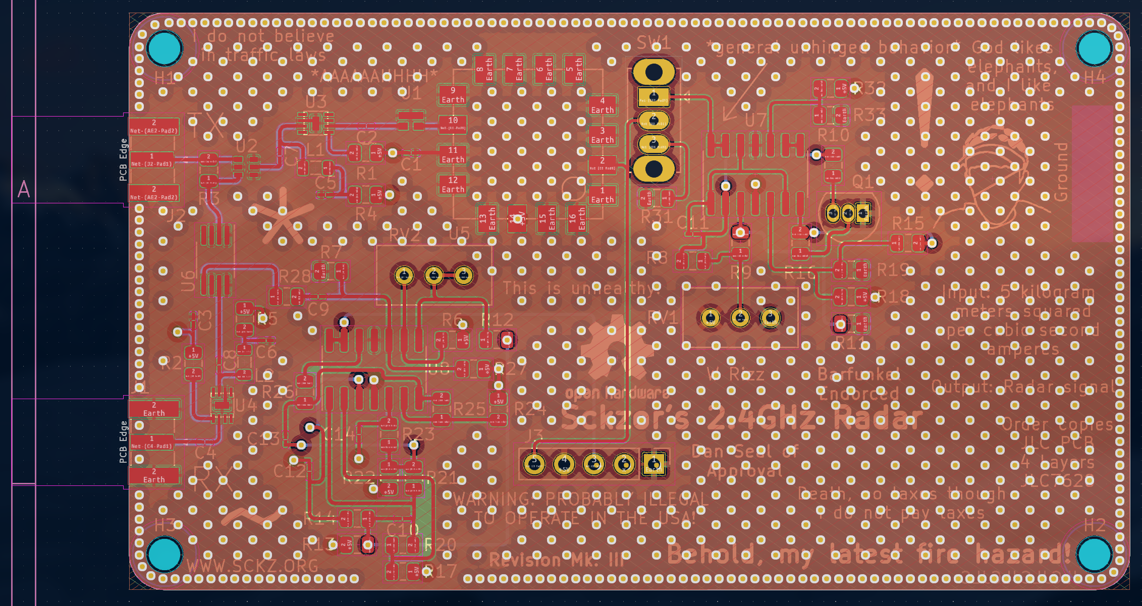
Above is the third version of the PCB. At the time of writing it is still being worked on. The main difference is that the components are all closer to each other in order to reduce interference. Additionally, there is much more grounding put in place in order to ensure that all of the components have solid access to the ground plane. One final minor change I made was that I moved the antenna taps to the opposite side of the board. This was because the USB port for the computer PCB that is designed to mount below the first board was originally positioned directly below them which made for rather awkward cable management.

The design files for all of these boards are available on my GitHub here if you would like one.

The second PCB that I dubbed the “Radar Computer” is much simpler than the first. It is simply a nice carrier board that holds a Raspberry Pi Pico in such a way that it can connect to the analog radar. The ramp and video amp signals both run into two of the analog input pins of the Pico in through a voltage divider (to convert the 5 volt radar signaling voltage to the 3.3 volts appropriate for the Pico.) The board also has a bit of standard perf-board space on the edge of it in case I want to add some extra circuitry to it. I eventually used some of it to make the I2C bus more accessible.

If you want one of these boards the design files are available on my GitHub here.

Software

The software for all parts of the project are written in my favorite programming language, C. All of the code is rather simple for anyone who have intermediate to advanced work with micro controllers so instead of focusing on what every line of code in my codebase does, I have released the codebase on my GitHub and I will write about the general implementation here. This will simultaneously allow you to write your own code in order to accomplish a similar feat as well as not boring anyone who wants to is a casual observer to death.

The code begins, as you might imagine, by performing initialization of the ADCs and bus ports on the Raspberry Pi. The code then begins polling the radar ports. It starts by waits for a known place within the radar’s ramp signal (in my case the peak of the triangle, but it could be anywhere). Once this happens it begins sampling the ADC that is connected to the video amp signal. This signal tends to be relatively high frequency, at least compared to the normal ADC sampling rate of a micro controller, so I had to push the Raspberry Pi a bit. I found a piece of code designed for high speed sampling of the ADCs on Alex Wulff’s GitHub page. By modifying this code slightly I was able to perform a sample for a given period of time and construct a surprisingly accurate wave form representing the received signal from my radar system.

When a radio signal hits an object it reflects at a different frequency depending on a variety of factors like the material, the distance, the speed and the angle of the object. These signals are reflected back to the radar system which measures them. This means that it is not really the waveform that we measure from the radar that is of concern to us, it is the frequencies that make it up that determine the different characteristics, most notably distance, above. The way the frequency composition of a waveform is determined is through use of a Fourier transform. This is the same algorithm used to determine the frequency composition of sound and basically every other waveform that needs to be decomposed. In order to execute this algorithm on a computer, especially a rather low power computer like the Raspberry Pi Pico, a variation of this algorithm is used called the Fast Fourier transform is used. It is basically a simple way to compute a Fourier transform and it is the method most commonly used. The implementation of this algorithm is relatively easy if you have taken pre-calculus level math and can be seen on the Wikipedia page (linked above) that undoubtedly explains it better than I ever could.

Once all of the mathematical signal processing is done the resulting frequencies are passed along over either the I2C or USB bus to another computer that can (hopefully) make used of the data. I wanted to try to offload as much computing to the onboard computer as possible in order to free any connected computer for other processing tasks, originally I was going to try to have a “higher accuracy” mode that allows the Raspberry Pi to act only as pipe to send information over a bus to a more powerful computer that could (presumably) perform calculations on much larger sets of data. However, as I experimented with different options for this I came to the realization that only USB would be fast enough to move that much data through the device without creating a worse bottleneck than with onboard processing. The code that would allow sending data over USB was quickly becoming very complex though and I wanted to save time to do other things, so this function will hopefully be coming at a later time.

I also wrote a small Linux driver that takes data from the I2C bus and registers an Industrial IO device with the kernel. The code for this driver can also be found on my GitHub in the same place as the rest of the code discussed. This driver is beyond the Scope of this post but suffice it to say that it is heavily based of Johannes 4GNU_Linux’s wonderful Let’s Code video.

Over all the software was not a complex as I imagined it would be, it actually ended up being rather simple and I wrote it in just a few days of work. It was nice to demystify how radar and similar hybrid analog/digital devices work.

Antennas

One integral part of the design for my radar system that I breezed over before because I couldn’t find a fluid way to fit it in was the antennas I used. In other small scale radar systems I saw mostly simple “cantennas” consisting of a small segment of wire inside a coffee can was used as the method for transmitting and receiving signals. I did not like the unoptimized nature of these antennas so I decided to cut my own antennas. I designed a yagi antennas based on some old 2.4 GHz WiFi antennas that I had lying around. They consist of a reflector/director element that was CNC cut from a sheet of scrap 16th inch aluminum as well as a small 1 layer PCB that serves as the driver element of the antenna. They are mounted within a waveguide made of a family sized can of Campbell’s Tomato Soup using a plastic bracket I had 3D printed. The driver elements are soldered to a piece of coaxial cable that attach to the antenna taps on the radar board for transmitting and receiving. I do not own any of the traditional “cantennas” nor the equipment needed to test the antennas against one another, so I have no proof that my antenna is any better or worse than those used by others, however, I would bet that my antennas are at the very least more directional, allowing more range out of my radar. All of the parts were designed in FreeCAD and KiCad and the design files are available on my GitHub in the Antennas folder in case you want to cut/3D print/etch some of your own. I will warn you I had quite the time trying to get the FreeCAD files into SolidWorks so they could be cut on the CNC router so any machining is at your own risk.

Acknowledgements

Thank you to radar_macgyver, Berni and everyone else who helped me with this project on the EEVBlog Forum. It would not have been possible without Them. Additionally, I want to thank Dan for discussing and reviewing my PCBs before I placed them into production. Finally, I would like to thank my parents for perpetually financing my strange endeavours. I am supremely thankful for these people, nothing that I accomplished here could have been done without them. Conclusion

This post just scratches the surface of all of the techniques, strategies and processes I learned in this project. When I started I could not possibly have imagined how much I would learn in the process of doing this. I would highly recommend anyone who has interest in this to try it, even if you fail you will learn lots.

Thanks for reading!